Soon after de Broglie introduced his hypothesis to the world, a period which is often referred to as the old quantum mechanics came to an end (1900 – 1925). The basic phenomena of the old quantum mechanics are the quantization of energy and the wave-particle duality. Since 1925 we are dealing with the modern quantum mechanics.
Austrian physicist Erwin Schrödinger in 1925 adjusts de Broglie’s inaccurate theory and assigns a so-called wave function to every quantum object. Temporal and spatial evolution of a wave function is described by a complex equation, the so-called Schrödinger equation. A wave function is denoted by the capital or lower-case Greek letter psi:
𝜳, 𝝍
The wave function is a complex mathematical function in which all the properties of a given quantum objects (momentum, position, etc.) are stored (this is different from the de Broglie’s matter wave, since de Broglie did not assign this property to his wave, moreover, he perceived the wave as a physical object, while Schrödinger’s wave function is merely abstract). This set of properties of a quantum object is called a quantum state. Quantum state is denoted as follows:
|𝝍⟩
The wave function is presumably the most significant idea of quantum mechanics, since most of the phenomena of the modern quantum mechanics are derived from it. Some of these phenomena, especially the principle of quantum superposition, are so different from the ones which are usual for us in the macroworld that it is often very difficult to believe, let alone understand them.
Quantum Superposition
Already when clarifying the phenomena of the old quantum mechanics, it became clear that the applicability of a certain phenomenon to the macroworld does not necessarily mean the applicability of this phenomenon to the microworld. One of the basic rules of the macroworld is that each object has only one position and one velocity. In other words, it is simply impossible to travel from Germany to the UK at 60 miles per hour while flying from Europe to Australia at eight times that speed. Astonishingly, this rule does not seem to apply to the quantum world, and objects from the microworld may therefore be in many places at once and do many things at once!
When conducting the double-slit experiment, an interference pattern is created only when a wave (wave function) from one slit interferes with a wave that passed through the other slit, as I have already described in the previous chapters. If we were to send waves (whether electromagnetic waves or matter waves) only through one slit, an interference pattern would not be created, of course. Let us imagine a situation where we are conducting the double-slit experiment with massive particles, such as protons, but with one small variation – we are sending only one proton at a time, so the wave functions of individual protons cannot interfere with each other. As strange as it may sound, even in this case, there is an interference pattern.
The entire classical physics is based on the idea of the so-called determinism. The basic principle of determinism is that the future is predictable and that the only thing necessary to predict the future evolution of the universe is having enough information about the present. For example, we can predict the next solar eclipse by having enough information about the motion of the Moon. The entire deterministic physics is based on this condition. Another idea of determinism is that identical conditions lead to identical results. For instance, if we were to shoot two identical bullets from a gun under the same conditions (i.e. in the same direction, at the same temperature, etc.), both bullets would hit the same place. However, the quantum world behaves completely differently. If we were to shoot electrons instead of bullets (from a hypothetical electron gun), each of these electrons could hit a different place and each of them could have a dissimilar velocity, even though the initial conditions were identical.
The strange behaviour of the protons from the second paragraph and the unpredictability of the electrons from the third paragraph are both a consequence of a crucial phenomenon of quantum mechanics – the principle of quantum superposition. Quantum superposition states that an object that is not being observed exists in all possible states at once – it is in a superposition. This superposition is a combination of all the states the object could theoretically be in. This means that a particle which is not observed can have multiple velocities and be at multiple places at once.
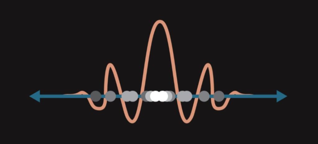
This may sound rather strange, but if we take the wave function into consideration, superposition starts to make sense. Consider, for instance, the position of an object. The wave function can be imagined as an abstract mathematical wave surrounding a given object. As mentioned before, the wave function contains all the properties of an object, the position of the wave function thereby determines the position of the object itself. This, however, poses a problem. Recall that a wave is not localized in space but instead tends to spread. This property applies to our wave function as well. It follows that as long as the wave function of an object exists, the position of this object is not fully defined and the object is basically located everywhere where its wave function is located. We say that this object is in multiple eigenstates. For a quantum object to have clearly specified position, the wave function must “disappear”. How to achieve that? Simply by observation.
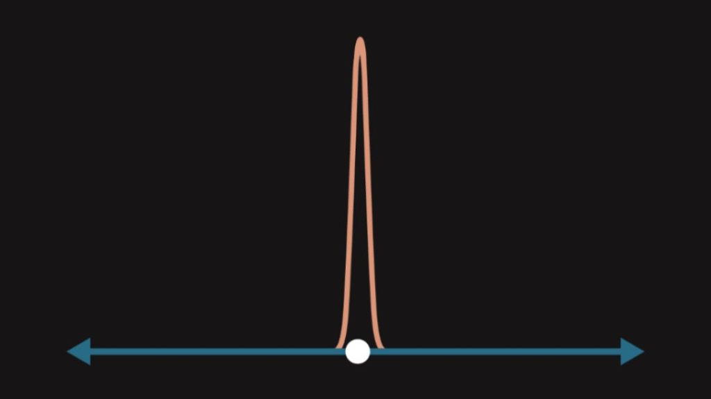
When a quantum object is observed, the so-called wave function collapse occurs. Wave function collapse is the reduction of the wave function to one eigenstate (one position, one velocity). Wave function collapse ensures that one can never observe an object with multiple velocities or positions, since the superposition is destroyed by mere observation. The act of observation thereby does not only identify the properties of a quantum object but also determines them! That basically means that we determine the future of an object purely by observing it (i.e. measuring its properties).
However, there is one important question: How does a quantum object select an eigenstate in which it is located when it is observed? This process is based on probability. The likelihood of a quantum object ending up in a certain eigenstate is determined by its wave function. The wave function is therefore also referred to as the probability wave. From each wave function, a complex number can be extracted, the so-called probability amplitude, which is used to determine this probability. The probability of a quantum object ending up in a certain eigenstate is determined as the square of the absolute value of the probability amplitude. If the probability of a certain process occurring is 50 percent, for instance, the probability amplitude of this process has a value of 𝟏/√𝟐.
Let us consider a situation where we want to ascertain the velocity of a certain electron. Let us say that this electron is in a quantum state that is a superposition of two eigenstates. The first eigenstate assigns the electron velocity 1, the second eigenstate assigns it velocity 2. This superposition of two velocities can mathematically be written as follows:
|𝛙⟩ = |𝐯𝐞𝐥𝐨𝐜𝐢𝐭𝐲 𝟏⟩ + |𝐯𝐞𝐥𝐨𝐜𝐢𝐭𝐲 𝟐⟩
As long as the electron is not observed, it has both velocities. The wave function assigns the electron a probability of ending in each of the eigenstates in case of observation. For illustration, let us assign the electron a 75 percent chance of ending up in the first state with velocity 1 and a 25 percent chance of ending up in the second state with velocity 2. Mathematically we can write this using probability amplitudes:
|𝛙⟩ = (3 / 4)-½ × |𝐯𝐞𝐥𝐨𝐜𝐢𝐭𝐲 𝟏⟩ + (1 / 4)-½ × |𝐯𝐞𝐥𝐨𝐜𝐢𝐭𝐲 𝟐⟩
If we now try to measure the velocity of the electron, its wave function collapses, and the electron obtains just one velocity. Let us say that in the first measurement, the electron has velocity 1. If we repeat the measurement multiple times using different electrons with the same wave function, we randomly get either velocity 1 or velocity 2. In 75 percent of the cases, the electron has velocity 1, in the remaining 25 percent of the cases, the electron has velocity 2. There is no way of knowing for sure which velocity the electron takes in the next measurement.
A quantum object can be in a superposition of an arbitrary number of eigenstates, and each of these states is assigned a certain probability value. The sum of probability values of all eigenstates of a quantum object in a superposition is equal to one. The probability of finding an object in one of its eigenstates is therefore always equal to 100 percent (in other words, if the object exists, it is always going to be somewhere – even though we may not be able to predict where). Mathematical notation (c1, c2, c3 are probability amplitudes):
|𝛙⟩ = 𝒄𝟏|𝐬𝐭𝐚𝐭𝐞 𝟏⟩ + 𝒄𝟐|𝐬𝐭𝐚𝐭𝐞 𝟐⟩ + 𝒄𝟑|𝐬𝐭𝐚𝐭𝐞 𝟑⟩ + ⋯
|𝒄𝟏|𝟐 + |𝒄𝟐|𝟐 + |𝒄𝟑|𝟐 + ⋯ = 𝟏
Let us now go back to the second and third paragraph of this chapter to understand what was happening. The proton in Young’s experiment is in a superposition, so it actually goes through both slits at once and interferes with itself! If we put a detector in front of the slits and observe which slit the proton goes through, its superposition is destroyed and the interference pattern disappears. The electron fired from a gun (the third paragraph) is in more eigenstates at once, and therefore has multiple velocities and is in multiple places at once. Only after the impact, when the wave-function collapse occurs, does the electron obtain just one position, which, however, does not have to be identical to positions of other fired electrons.
We do not encounter superposition on a daily basis, since objects from the macroworld continuously interact with their environment which acts as an observer, and therefore wave function collapse occurs constantly.
Quantum superposition is an elementary principle of quantum mechanics. It breaks the deterministic perception of the world. In quantum mechanics, future is determined only within probabilities, and the same conditions often lead to utterly different results.
One might think that probability is present in the macroworld as well. However, the opposite is true. Any seemingly random phenomenon from the macroworld, throwing a dice, for instance, is completely deterministic and any “randomness” is caused purely by our insufficient knowledge of the system. In the case of throwing a dice onto a surface, it is the height of the dice above the surface, the speed of the rotation of the dice, the mass of the dice, the surface roughness of the table, and so on. If we had a powerful supercomputer that would be able to take all these factors into consideration, we would know exactly which value the dice would show at any given time.
This, however, does not hold true in the microworld. In quantum mechanics, instead of the question: “Where is a particle located?” we ask the question: “What is the probability of finding a particle in a certain place?”
Schrödinger’s Cat and Interpretations of Quantum Mechanics
There is no doubt that quantum mechanics is a revolutionary and an exceptionally strange theory. After the establishment of the modern quantum mechanics, physicist divided themselves into several opinion groups. Each of these groups tried to explain the weirdness of the quantum world in a different way, which led to the creation of many interpretations of quantum mechanics. The most acknowledged of these interpretations is the so-called Copenhagen interpretation (this interpretation was used in the previous chapter). Another very interesting interpretation is the so-called many-worlds interpretation. We can demonstrate the difference between these two interpretations on a simple thought experiment.
Let us say we have a box in which an atom of a radioactive element is located. A radioactive element is an element that undergoes decay to lighter elements in a certain period of time. The problem is that one can never know when the decay occurs, since each radioactive atom is described by a wave function that determines only the probability of the atom decaying over time. The probability of the decay occurring increases with time. Thus, the so-called half-life was defined. Half-life is the amount of time after which the probability of an atom decaying is exactly 50 percent. Each radioactive element has a different half-life (ranging from fractions of a second to millions of years). For instance, if we had 100 atoms of an element with a half-life of one year, 50 atoms would have decayed after one year.
Let us go back to our atom in a box. For simplicity, suppose that the half-life of our radioactive element is one day, i.e. if we leave the atom in the box for one day, there is a 50 percent probability of it decaying. However, recall that unless a quantum object is observed, it is in a superposition of all possible states. Therefore, the atom is both decayed and not decayed. In other words, our atom isolated inside of the box is in a superposition of two states – decayed / non-decayed. Only when we open the box and observe the atom, does the wave function collapse occur and the atom “decides” whether it is decayed or not decayed based on the probability given by its wave function (after one day, this probability is 50 percent for both decayed and non-decayed state). Now let us consider a situation where we put a vessel full of poisonous gas and a living cat in the box along with the atom. The whole system is set up so that if the decay occurs, the poisonous gas is released and the cat dies. If the atom does not decay, the gas is not released and the cat stays alive.
If this thought experiment seems familiar to you, it is because we are dealing with the most famous “paradox” of quantum mechanics. The author of this thought experiment is a famous physicist Erwin Schrödinger, the experiment is therefore often referred to as Schrödinger’s cat. With this experiment, Schrödinger wanted to demonstrate the vagueness of the Copenhagen interpretation. It bothered him that the Copenhagen interpretation does not clearly define what it means to “observe” a quantum object. According to him, the Copenhagen interpretation basically says that if an atom is in the superposition decayed/non-decayed, the poison is in the superposition released/not released, which implies that the cat is in the superposition alive/dead until the box is opened. The cat obviously cannot be dead and alive simultaneously. That is why Schrödinger considered the Copenhagen interpretation silly.
However, the authors of the Copenhagen interpretation themselves never saw Schrödinger’s cat as a problem, since they reckoned that the fate of the cat is decided long before the box is opened, since atoms in the air around the radioactive atom “observe” (bump into) it and thereby prevent superposition of the cat. Even the cat herself can observe whether the poisonous gas is released or not, therefore preventing superposition.
Each interpretation explains Schrödinger’s cat a little differently. For instance, the aforementioned many-worlds interpretation assumes that every time two quantum systems interact, the reality is split into multiple parallel “worlds”. The interaction leads to different results in each of these worlds. In other words, everything that can happen does happen in at least one of the worlds. This means that when the box is opened, the whole universe splits into two universes, one of them containing a living cat, the other one containing a dead one!
